
If you’ve ever stared at a massive spreadsheet trying to spot the one number that matters, you already know why conditional formatting exists. It’s one of Excel’s most underrated features — quiet, unassuming, and yet capable of turning a wall of numbers into a story you can read in seconds.
This guide walks you through conditional formatting from the ground up: what it is, why it matters, where to find it, and how to actually use it for real-world tasks like highlighting rows, spotting blanks, and cleaning up rules you no longer need. By the end, you’ll be comfortable enough to start experimenting on your own data.
What is Conditional Formatting in Excel?
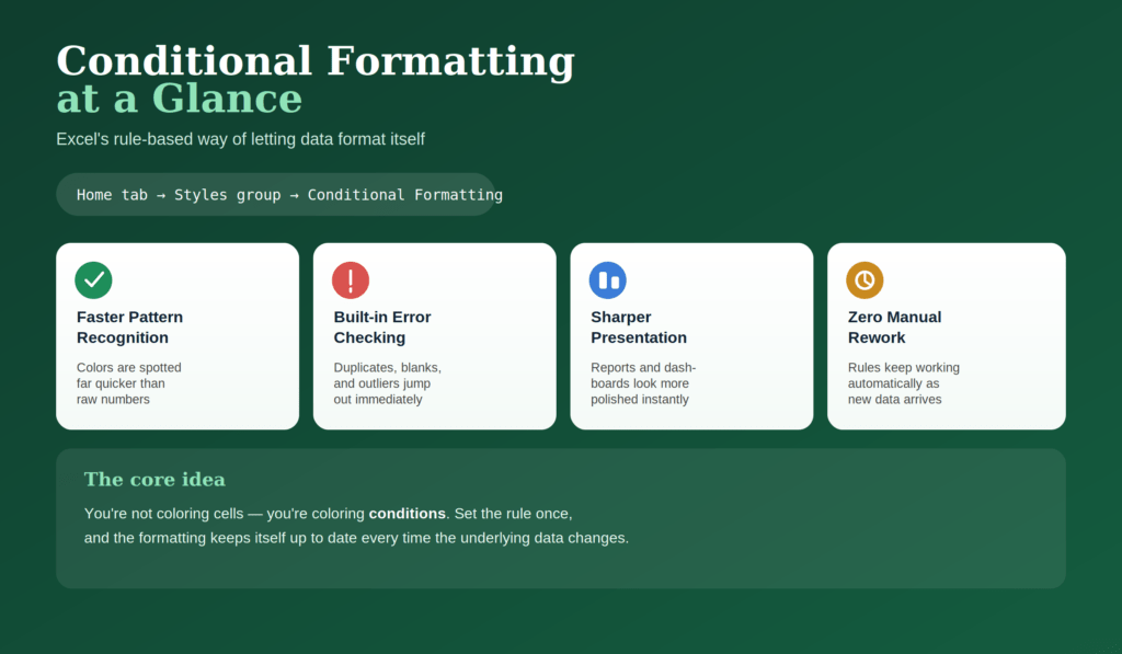
At its core, conditional formatting is Excel’s way of letting your data format itself. Instead of manually coloring cells one by one, you set up a rule — “if this condition is true, apply this style” — and Excel takes care of the rest, automatically and dynamically, every time your data changes.
The “formatting” part can mean several things:
- Changing the font color or making text bold/italic
- Filling a cell with a background color
- Adding data bars, color scales, or icon sets
- Applying borders
The “conditional” part is simply the rule that triggers it — a value being above average, a date falling in the past, a cell being empty, or a custom formula you write yourself.
The real power here is that this formatting isn’t static. If the underlying data changes, the formatting updates instantly. You’re not coloring cells; you’re coloring conditions.
Why Use Conditional Formatting in Excel?
It’s tempting to think of conditional formatting as decoration, but it’s really a data analysis shortcut. A few concrete reasons it’s worth learning properly:
- Faster pattern recognition — Your eyes catch color changes far quicker than they scan raw numbers.
- Built-in error checking — Duplicate entries, missing values, and out-of-range figures jump out immediately instead of hiding in a sea of digits.
- Better presentation — Reports and dashboards look more polished and professional when key figures are visually emphasized.
- Less manual work — Once a rule is set, you never have to reformat the sheet again, even as new data rolls in.
In short, it does the first pass of analysis for you, so you can spend your time interpreting the data instead of hunting for it.
Where to Find Conditional Formatting in Excel?
Good news: this feature hasn’t moved around much across Excel versions. Whether you’re using Excel 2010, 2016, 2019, or Microsoft 365, you’ll find it in the same place:
Home tab → Styles group → Conditional Formatting
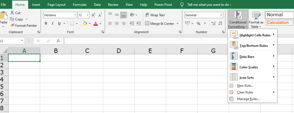
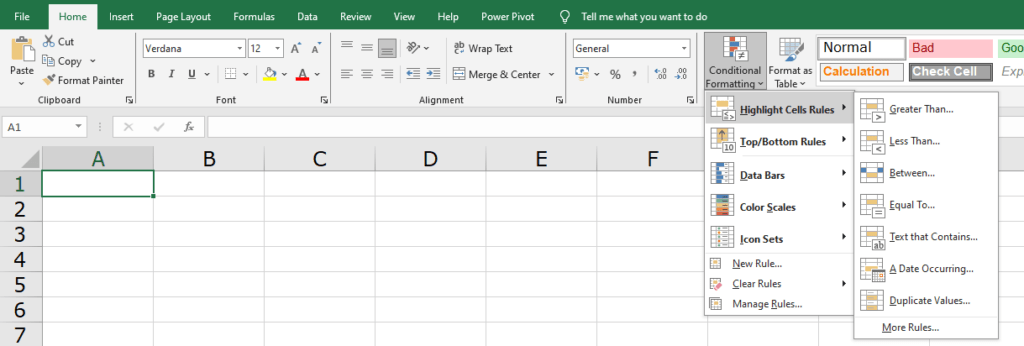
Click that dropdown and you’ll see a menu with several categories — Highlight Cells Rules, Top/Bottom Rules, Data Bars, Color Scales, Icon Sets, and a New Rule option for anything custom. The layout is nearly identical across versions, so once you learn it here, you’re set no matter which Excel your office (or your client) happens to run.
How to Apply Conditional Formatting in Excel?
Getting started doesn’t require any formulas at all. Here’s the basic flow:
- Select the range of cells you want to format.
- Go to Home → Conditional Formatting.
- Pick a built-in rule (for example, “Highlight Cells Rules → Greater Than…”) or choose New Rule for something more specific.
- Set your condition and choose a formatting style.
- Click OK.
That’s it. Excel immediately scans the selected range and applies the formatting wherever the condition is met — and keeps checking every time the data updates.
Once you’re comfortable with the built-in rules, the real flexibility comes from writing your own formulas, which is what the rest of this guide focuses on.
How to Highlight an Entire Row Based on One Cell’s Value
Highlighting a single cell is useful, but often you want the whole row to stand out — for example, flagging every order that’s been “Shipped” or every employee marked “Inactive.” This requires a small formula-based rule instead of a built-in one.
Here’s how to do it:
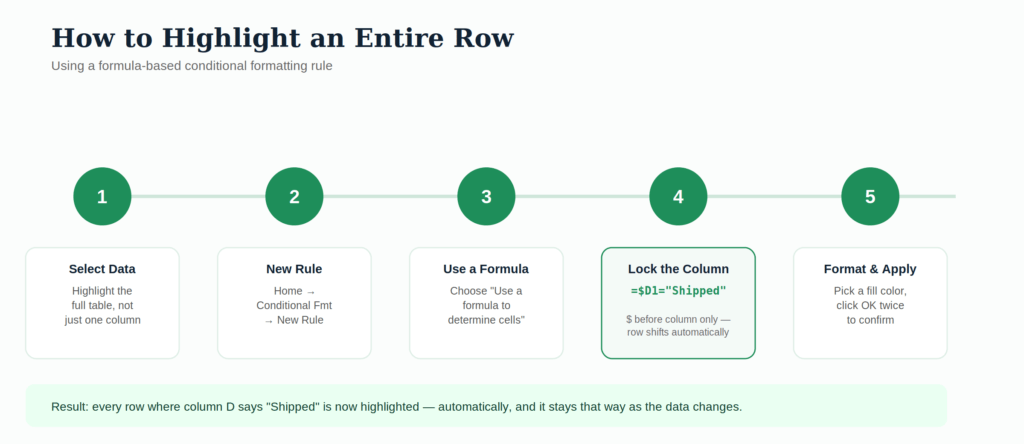
- Select the full range of data you want the formatting applied to (not just one column — the entire table).
- Go to Home → Conditional Formatting → New Rule.
- Choose “Use a formula to determine which cells to format.”
- Type a formula that references the first row of your selection, and lock only the column with a single dollar sign. For example, if column D contains a status and you want to highlight rows marked “Shipped”:
=$D1=”Shipped”
- Click Format, pick a fill color or font style, and confirm.
- Click OK twice to apply.
The key detail beginners often miss is the dollar sign placement. $D1 locks the column but lets the row shift as Excel checks each row in your selection — which is exactly what makes the whole row light up together, instead of just one cell.
How to Copy Conditional Formatting in Excel?
Once you’ve built a rule you like, you don’t need to recreate it from scratch elsewhere. There are three simple ways to reuse it.
01.Using Conditional Formatting Rules Manager:
This copies just the rule itself, without touching any other formatting on the cell.
Go to Home → Conditional Formatting → Manage Rules.
Set “Show formatting rules for” to This Worksheet.
Select the rule you want to duplicate and click Duplicate Rule.
Edit the cell reference on the duplicated rule to point to your new range.
Click OK.
02. Using Format Painter:
This is the fastest option when you just want to “paint” the same formatting somewhere else.
- Click a cell that already has the formatting.
- Click Format Painter on the Home tab (the little paintbrush icon).
- Drag across the new cells where you want it applied.
03. Using Paste Special Option with Keyboard Shortcuts:
This copies everything about the cell’s formatting, conditional rules included.
- Copy the source cell (Ctrl+C).
- Select the destination cells.
- Right-click → Paste Special → choose Formats → OK.
Each method has its use case: Rules Manager is best for precision, Format Painter for speed, and Paste Special when you’re already copying other formatting anyway.
How to Edit Conditional Formatting in Excel?
Rules rarely stay perfect forever — thresholds change, new categories get added, priorities shift. To update a rule:
- Click any cell inside the formatted range.
- Go to Home → Conditional Formatting → Manage Rules.
- Select the rule you want to change and click Edit Rule.
- Adjust the condition or the formatting, then click OK.
If you have multiple rules stacked on the same range, the Rules Manager also lets you reorder them using the Move Up / Move Down arrows — this matters because Excel applies rules in the order listed, and a higher rule can override a lower one if both conditions are true at once.
How to Remove Conditional Formatting in Excel?
Sometimes the cleanest fix is to start over. To clear rules:
- Select the cells (or the whole sheet) you want to clean up.
- Go to Home → Conditional Formatting → Clear Rules.
- Choose either:
- Clear Rules from Selected Cells — removes formatting only from what you’ve selected.
- Clear Rules from Entire Sheet — wipes every conditional formatting rule on the sheet, regardless of what’s selected.
Use the “entire sheet” option carefully — it’s easy to accidentally remove rules you’d forgotten about elsewhere on the same tab.
How to Use Conditional Formatting in Excel to Highlight Blank Cells?
Empty cells are often the most important thing to catch — a missing invoice number, an unanswered survey question, an incomplete form. Excel gives you two ways to flag them.
Option 1: The Built-In Blanks Rule
- Select your range.
- Go to Home → Conditional Formatting → New Rule.
- Choose “Format only cells that contain.”
- From the dropdown, select Blanks.
- Choose your formatting (a red fill works well for visibility) and click OK.
This is the quickest route and works well for simple, one-off checks.
Option 2: The ISBLANK() Formula
For more control — say, you want blank cells highlighted only if another related cell has data — a formula gives you flexibility the built-in rule can’t:
- Select your range.
- Go to Home → Conditional Formatting → New Rule → Use a formula to determine which cells to format.
- Enter a formula like:
=ISBLANK(D3)
(Adjust the cell reference to match the first cell in your selected range.)
- Set your formatting and click OK.
The formula approach is worth learning early, because once you understand ISBLANK(), you can combine it with AND() or OR() to build much smarter blank-detection rules — for example, flagging a row only if it’s blank and the order was marked “Pending.”
A Few Practical Tips Before You Go
- Formula rules always start with =. If Excel treats your formula as plain text instead of a rule, check for a stray space or a missing equals sign.
- Absolute vs. relative references matter more here than anywhere else in Excel. A single misplaced $ sign is the most common reason a row-highlighting rule only formats one column instead of the whole row.
- Rule order is not automatic priority by importance — it’s top-to-bottom in the Manager, so put your most specific rules above your general ones.
- Too many overlapping rules will slow down large sheets. If your workbook feels sluggish, check Manage Rules for duplicate or conflicting entries you can consolidate.
- Conditional formatting doesn’t change the actual data — only its appearance. It’s completely safe to experiment with, since you can always clear a rule without affecting a single number underneath it.
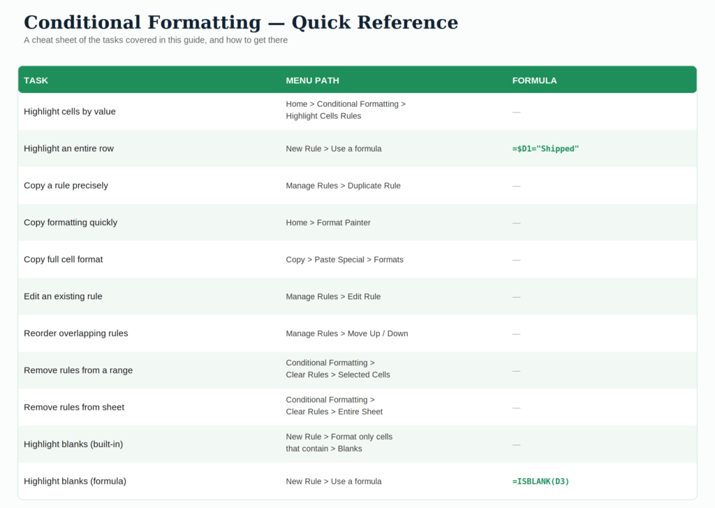
Wrapping Up
Conditional formatting is one of those Excel features that feels optional right up until you use it properly — and then you wonder how you ever managed a spreadsheet without it. Start simple: highlight a few cells based on value, then work your way up to formula-based rules for entire rows and blank-cell detection. Once those two techniques feel natural, you’ll find yourself reaching for conditional formatting on almost every sheet you build, because it turns raw numbers into something you can actually see — and that’s the whole point of a spreadsheet in the first place.