Welcome to my guide on mastering Excel errors! If you’ve ever felt the frustration of encountering errors while working in Excel, you’re not alone. From #REF! errors to formula mistakes, Excel can sometimes feel like a minefield of potential pitfalls. But fear not! In this comprehensive blog post, I’ll take you from frustration to fix, providing you with the knowledge and tools you need to conquer common Excel errors like a pro.
Understanding Common Excel Errors
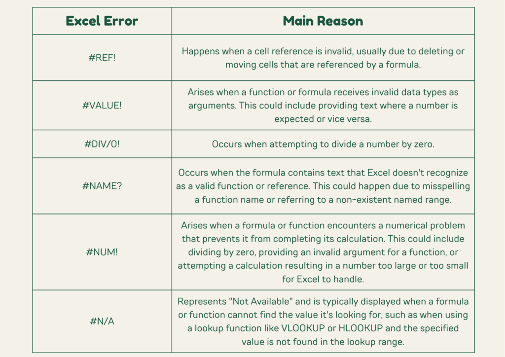
#ref error in Excel
This error occurs when a formula references a cell that doesn’t exist or is invalid. For example, if you delete a cell that a formula depends on, Excel can’t find the cell anymore, resulting in a #REF! error. It’s like asking someone for directions to a place that no longer exists.
#value error in Excel
This error arises when a formula includes invalid data types or operations. For instance, if you try to add text to a number using the SUM function, Excel doesn’t know how to handle it and returns a #VALUE! error. It’s like trying to add apples and oranges together—it just doesn’t work!
#div/0 error in Excel
This error occurs when you attempt to divide a number by zero, which is mathematically undefined. For example, if you have a formula dividing a value by zero, Excel can’t perform the calculation and returns a #DIV/0! error. It’s like trying to split a pizza among zero people—impossible!
#name error in Excel
In Excel, “#NAME?” error occurs when the formula contains text that Excel doesn’t recognize as a valid function or reference. This could happen due to various reasons such as misspelling a function name, referring to a non-existent named range, or using a function that isn’t available in your version of Excel. It’s essentially Excel’s way of saying “I don’t recognize what you’re trying to do.”
#num error in Excel
The “#NUM!” error in excel occurs when a formula or function encounters a numerical problem that prevents it from completing its calculation. This could happen due to various reasons such as dividing by zero, providing an argument that’s not valid for a function, or attempting to perform a calculation that results in a number too large or too small for Excel to handle.
#N/A error in Excel
In Excel, the “#N/A” error stands for “Not Available.” It occurs when a formula or function cannot find the value it’s looking for. This error commonly appears when using lookup functions like VLOOKUP, HLOOKUP, MATCH, or INDEX-MATCH, and the specified value is not found in the lookup range.
Strategies for Resolving Excel Errors:
Here is a step-by-step guide to troubleshooting Excel errors
How to fix a #REF! error in Excel
To fix a #REF! error, you need to identify which cell or range is causing the error and adjust the formula to reference a valid cell or range. This may involve restoring deleted cells, correcting cell references, or updating formulas to include the correct range.
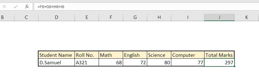
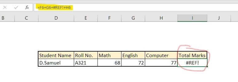
Here the above example total marks 297 calulated by adding four subject marks . Now any subject column wrongly deletes the #REF! error will appear like the following image ;
- Case #1: Invalid Cell Reference:
- The #REF! error occurs when you reference a cell that doesn’t exist or has been deleted.
- For example, if you have a formula like
=A1+B2and either cell A1 or B2 is deleted, you’ll encounter this error. - To fix this, ensure that all cell references in your formulas are valid and point to existing cells.
- Case #2: Incorrect Range Reference:
- If you’re using a range reference (e.g.,
SUM(A1:A10)), make sure the range covers valid cells. - If you accidentally delete or move cells within the range, Excel will throw a #REF! error.
- Double-check your ranges and adjust them as needed.
- If you’re using a range reference (e.g.,
Pro Tip: To eliminate the #REF! error, always ensure that when using a formula between two sets of data on different sheets or workbooks, utilize the “Paste Special Values” option in Excel before sharing the output data file with others. This helps to retain the calculated values without maintaining the formula references, thus preventing potential errors when the file is accessed by different users.
How to fix #value error in Excel
The #VALUE! error in Excel can be quite frustrating, but fear not! Let’s unravel the mystery and learn how to tackle it like an Excel pro.
Case #1: Wrong Data Type:
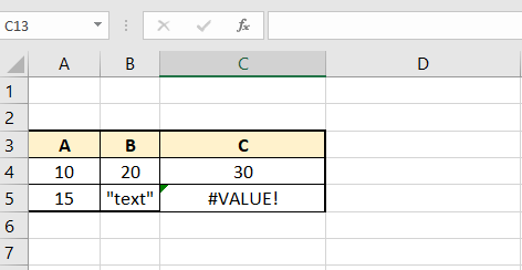
This error often occurs due to incorrect data types in cell references. For instance, if you’re trying to add numbers from cells A4 to B4, and cell A5 to B5, you’ll notice that cell B5 contains a value like “text”
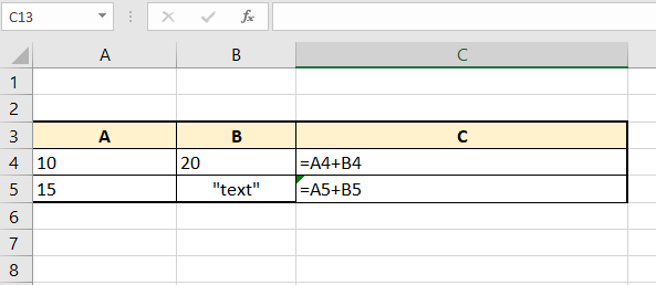
Now, let’s look at the formulas in Column C:
=A4+B4: This formula in cell C4 adds the values from cells A4 and B4. Since both A4 and B4 contain numeric values, the formula executes correctly and produces the result 30. Whereas,
=A5+B5: This formula in cell C5 tries to add the values from cells A5 and B5. However, B5 contains the text “text”, which is not a numeric value. Excel cannot perform arithmetic operations on text, so it returns a #VALUE! error because it cannot interpret the text as a number.
When you encounter a #VALUE! error in Excel, it’s important to check your formulas and ensure that all the referenced cells contain compatible data types for the operation you’re trying to perform. In this case, converting the text to a numeric value or using an appropriate function to handle text data would resolve the error.
Case #2: Empty Cells Not Truly Blank:
Sometimes, empty cells aren’t genuinely blank. Hidden spaces or other non-visible characters can cause the #VALUE! error.
Example:
Suppose you’re dividing column B by column A. If cell B3 is empty (but not truly blank), you’ll encounter the error.
To fix this, ensure that empty cells are genuinely empty (no hidden characters) or handle them appropriately in your formulas.
How to fix #div/0 error in Excel
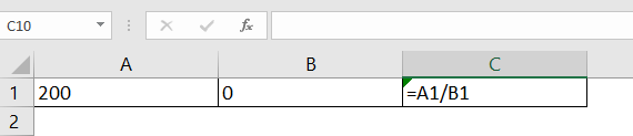
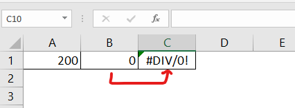
Imagine you have a simple Excel sheet where you’re dividing numbers in column A by numbers in column B. Sometimes, the numbers in column B are zero, which causes the #DIV/0! error.
Here’s how you can fix it using a simple trick: Using the IFERROR Function
Understand the Formula: Your division formula might look like =A2/B2, where A2 is the dividend (number to be divided) and B2 is the divisor (number to divide by).
Apply IFERROR Function: To fix the error, you can wrap your division formula within the IFERROR function.
=IFERROR(A2/B2, "Oops! Can't divide by zero")
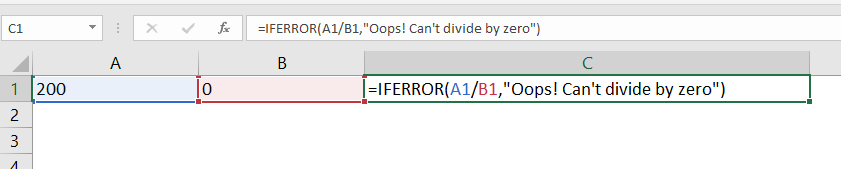
This formula says, “If there’s an error when dividing A2 by B2 (like dividing by zero), show the message ‘Oops! Can’t divide by zero’ instead of the error.”
Drag the Formula Down: Now, drag this formula down along the cells where you’re performing the division. Excel will automatically adjust the cell references for you.
How to fix #name error in Excel
Here’s how you can fix the #NAME? error:
Check Spelling:
Make sure you’ve spelled the function or formula name correctly. Excel functions are not case-sensitive, but they must be spelled correctly.
Verify Function Availability:
Ensure that the function or formula you’re using is available in your version of Excel and is supported by your language settings. You can consult Excel’s documentation or online resources to check for function availability.
Example:
Let’s say you’re trying to use the VLOOKUP function to search for a value in a table. If you accidentally misspell it as VLLOKUP, you’ll encounter the #NAME? error. Here’s how you can fix it:
Incorrect Formula:
=VLLOKUP(A2, Table1, 2, FALSE)
Corrected Formula:
=VLOOKUP(A2, Table1, 2, FALSE)
Pro Tips:
Use Function AutoComplete When typing a function or formula name, Excel provides autocomplete suggestions. This can help prevent spelling errors.
How to fix #num error in Excel
Check for Invalid Numerical Values:
Ensure that your formulas don’t contain any operations that result in invalid numerical values, such as division by zero or square root of negative numbers. For example:
Avoid: =A1/0 or =SQRT(-1)
Instead, check your data and adjust the formula accordingly to avoid these invalid operations.
Verify Function Arguments:
Make sure you’re using functions with the correct arguments and parameters. For instance:
Ensure that the INDEX function is supplied with valid row and column numbers.
Verify that the LOG function has positive numeric arguments.
Handle Extreme Values:
If your calculations involve very large or very small numbers, Excel may return a #NUM! error. Consider scaling down or scaling up your values or using alternative approaches to handle such cases.
Example:
Let’s say you have a data like this;
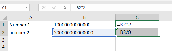
In this table:
Column A contains labels for the numbers.
Column B contains very large numbers.
Column C contains formulas to perform calculations on these numbers.
Now, let’s examine the formulas in Column C:
=B2*2: This formula in cell C2 multiplies the value in B2 by 2. Since B2 contains a very large number, the result of this multiplication could also be very large. If the result exceeds Excel’s numerical limits, it may lead to a #NUM! error.
=B3/0: This formula in cell C3 attempts to divide the value in B3 by 0. Dividing by zero is mathematically undefined, so Excel returns a #NUM! error in this case.
To handle extreme values and avoid #NUM! errors in such cases, you can consider scaling down the numbers (e.g., representing them in a different unit or using scientific notation) or using alternative approaches in your calculations. For example, you might avoid dividing by zero or use conditional logic to handle such cases gracefully.
How to fix #N/A error in Excel
Check Lookup Value Existence:
The #N/A error often occurs with functions like VLOOKUP, HLOOKUP, LOOKUP, or MATCH.
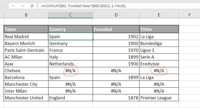
If a formula can’t find the value it’s looking for, it triggers this error ( See the above screenshot).
look at this screenshot image where Vlookup formula didn’t find the “Chelsea” lookup term in source data ( Football Data table), so you get #N/A error.
Solution:
Make sure the lookup value exists in the source data.
Otherwise, Use the IFERROR function to handle errors:
Example: =IFERROR(FORMULA(), ” “) (If the formula has an error, it displays nothing or is blank; otherwise, show the result).
Example:
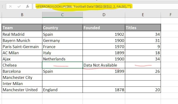
Suppose you’re using VLOOKUP to find the team country and the year it was founded from the Football Data table. If the team name isn’t found, you want to see nothing or blank or like “Data Not Available” instead of getting #N/A error.
To handle it, use: =IFERROR(VLOOKUP($B8, ‘Football Data’!$B$2:$E$12, 2, FALSE),””)
Or use
=IFERROR(VLOOKUP($B8, ‘Football Data’!$B$2:$E$12, 2, FALSE),”Data Not Available”)
From the dreaded #VALUE! to the mysterious #NUM!, each error holds valuable lessons. Take a deep dive into your formulas, ensuring they speak the same language and play nice with each other. When faced with colossal numbers or tricky divisions, consider a little scaling magic or a dash of creative problem-solving. Embracing these challenges not only conquers frustration but also boosts your Excel prowess, turning you into a confident spreadsheet wizard. So, don’t fear the errors—embrace them as stepping stones to mastering Excel like a pro!