How to Freeze a Row in Google Sheets

Boss:  Show me your data 

Employee: Here it is sir

Boss: 😣where is the heading of your data?

Employee: Sir… you must scroll up the sheet to view the header row!

Boss: why don’t you freeze the heading of your data….???

Do you ever face such a situation in the office, then you must know how to freeze a row in Google Sheets or any spreadsheets.

What is Freezing Rows?

Freezing rows in Google Sheets allows you to keep certain rows visible at all times, even when you scroll down the spreadsheet. This can help keep headings, labels, or other important information in view as you work with your data.

How to Freeze a Row in Google Sheets

There are two ways to freeze rows in Google Sheets:

Method 1: Using the View Menu

• Select the row you want to freeze.
• Click on the View menu at the top of the screen.
• Select Freeze.
• Choose the number of rows you want to freeze.

Method 2: Using the Drag-and-Drop Method

• Click on the Hand icon in the top left corner of the spreadsheet.
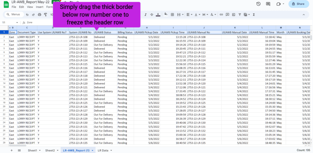
• Drag the thick horizontal line below the row number one or the row you want to freeze( see the above image).
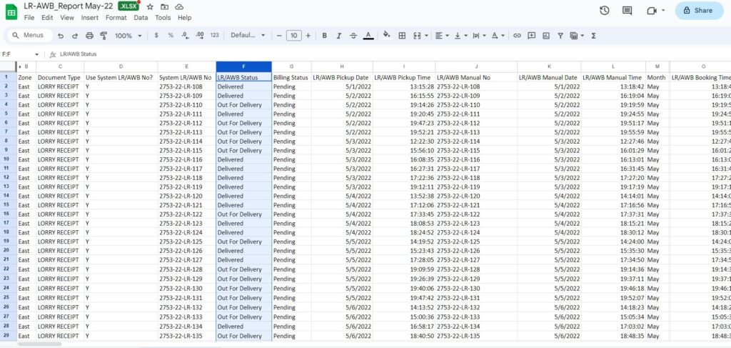
• Now the header row is frozen as you see in the below image.

How to unfreeze a row in Google Sheets

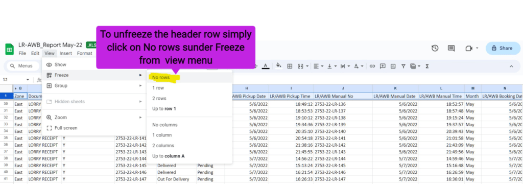
To unfreeze rows, simply follow the same steps and select No rows from the Freeze menu as you see in the below image.

Benefits of Freezing Rows

Freezing rows can provide a number of benefits, including:

• Keeping important information visible at all times
• Making it easier to navigate large datasets
• Reducing the need to scroll back and forth
• Improving data entry accuracy

Examples of When to Freeze Rows

There are a number of situations where freezing rows can be helpful. For example, you might want to freeze rows:

• When working with a spreadsheet that has a lot of data
• When using a spreadsheet for data entry
• When creating a report or presentation
• When collaborating on a spreadsheet with others

Tips and Tricks

Here are some additional tips and tricks for effectively using the freeze feature in Google Sheets:

Freeze Multiple Rows:

You’re not limited to freezing just one row. If you have several rows you want to keep visible, you can select “2 rows” or use the “Up to current row” option to freeze multiple rows at once.

Freeze Columns:

 In addition to freezing rows, you can freeze columns. This is useful if you have a lot of columns, and you want to keep some of them visible as you scroll horizontally. To do this,

First select a column instead of a row, here I select column F as you see in the below image

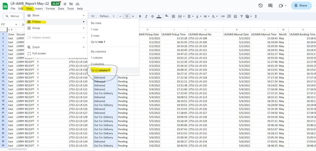
Second use the “Freeze” option from View menu accordingly as mentioned in below image

Combine Freezing:

You can freeze both rows and columns simultaneously to keep a specific area visible while scrolling in both directions. This can be very helpful when working with large datasets.

Avoid Over-Freezing:

While freezing rows and columns, be mindful not to overdo it. Excessive freezing can clutter your sheet and make it challenging to work with. Only freeze the rows and columns that are truly necessary for your workflow.

Scrollbars:

When you have frozen rows or columns, Google Sheets will add horizontal and vertical scrollbars if your data extends beyond the visible area. You can use these scrollbars to navigate your sheet while keeping your frozen rows or columns in view.

Mobile and Tablet Use:

If you’re using Google Sheets app on a mobile device or tablet, the freeze feature may work slightly differently. Check the app’s documentation or settings for specific instructions on how to freeze a row in the Google Sheets app.

Conclusion

Freezing rows is a simple but powerful feature that can make working with Google Sheets even more efficient. By following the steps above, you can easily freeze rows in your Google spreadsheets and reap the benefits of this useful tool.

Remember to use this feature wisely, striking a balance between keeping essential data in view and maintaining a clean and organized spreadsheet. As you become more proficient with Google Sheets, you’ll find that freezing rows is just one of the many tools that can help you master your data management tasks.