
If you are a spreadsheet user and frequently use spreadsheets for MIS work of your office task or any data-related work you might be using vlookup function in Excel. Today I’ll show you how you can use vlookup in Google Sheets to do your task with ease and share completed tasks with your boss or colleagues easily.
Vlookup is a very powerful function built-in Google’s popular spreadsheet application Google Sheets. Vlookup or “vertical lookup” takes advantage of vertically aligned data ranges or tables to easily locate data associated with a given value.
Let’s take an example to understand why vlookup function you should learn;
Here two table of HR data is given: Table1 & Table2, you need to make a report by adding a new column called Employee ID with Table1 data. How to do that?

Now, you are thinking that you can do this by simply copy the column “Employee ID” from Table 2 and paste it to the right of Table 1, that’s so easy.
Yes, you can do that for this tiny data, but if you have 1000 or 10000 or more employee data, and both tables not having the same set of data how can you do it immediately? Is it that easy?
Again a big yes if you do it by using the VLOOKUP function.
Let’s do it step by step……
Step 1 :
Please make sure that the common data field in both tables is at the extreme left of the Table. Here in these two data tables, the common field is the NAME column and is at the extreme left.
Step 2:
For output report add a separate column at the extreme right of Table 1 with the same formatting and name it “Employee ID”.
Select cell E31 of the output table and type the VLOOKUP function in the cell.

Step 3:
In the VLOOKUP function four criteria need to provide, they are:
1. Search Key :
It means which data you want to match to get the required data. In this example, we need to get the employee Id of MR.A.So search criteria are the cell number (A31) of MR.A.
2. Ranges:
It means from which data range you want to get the required data. Here you need to get employee ID from Table 2 data, so select A10:D13 Table 2 except the heading of the table and fix the range using $ sign ($A$10:$D$13).
3. Index :
It means In which of the Index/column the required data is present. Here” Employee ID“is column number 2.
4. is_Sorted (Optional Key) :
And the optional key is TRUE or FALSE, by default it is True or if you are not mentioned in a formula it is assumed as true, but it is recommended to set it as False because it returns an exact match. Here I have used the False key for the exact match.
Step 4:

Drag the cursor from E31 to E34 to complete the task.
So by using the VLOOKUP function you can do it within 1 minute.
Sometimes it is possible that some data doesn’t match exactly as both tables have different sets of data, in that case, the VLOOKUP function gives # N/A error, which means some data is not matched between both tables.

If you collaborate or share this output report with your boss it looks unprofessional due to #N/A error, Isn’t it?
So here is the solution that makes a perfect report for you.
Here you can use =IFNA () function along with Vlookup as the screenshot displayed below :


It gives you the output report like this :

Conclusion :
You have learned the basic Vlookup function and Ifna function to generate a professional report. And remember that the Vlookup function is one of the most powerful functions. If you combine another function with it, it is called advanced Vlookup formulas that can generate exceptional dynamic reports within a few minutes.
If you like this article helpful please make your comment and share it with your friends, also give your valuable suggestions for future articles.
Can VLOOKUP be done on Google Sheets?
Yes, you can use the Vlookup formula on google sheets to find related values or text from data sets in the same google sheets or from other sheets.
What is better than VLOOKUP in Google Sheets?
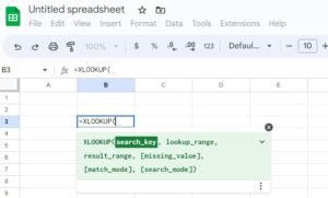
The best alternative Vlookup function in Google Sheets is Xlookup which is included in Google Sheets in the year 2022. The arguments of the Xlookup function are easier to use than Vlookup.
Why google sheets vlookup not working?
There could be many reasons why VLOOKUP is not working in Google Sheets. The most common reason may be there are unwanted trailing spaces in the cell that fails to find the search value.Use the TRIM function to remove trailing spaces or you can use the CLEAN function to delete all non-printing characters to solve this problem. Another reason could be the incorrect number formatting. This means that the format of the cell with a required value and the format of the leftmost column in the search range are different. you can simply fix it by changing the cell’s number format. Select the cell and go to Format Number Plain text in the Google Sheets menu. Its contents will be changed into the text. That will cause the error to be gone since you’ll be looking for the text string among other text strings.