Google Sheets is a powerful spreadsheet tool for managing and analyzing data, and one of its most useful functions is SUMIF. In this article, I will explain how to use  SUMIF in Google Sheets to calculate sums based on specific criteria. Whether you’re a beginner or an advanced user, this detailed article will guide you to unlock the full potential of the google sheets SUMIF function easily.

What is the SUMIF function?

As the name suggests SUMIF means sum if a certain condition matches. The SUMIF function in Google Sheets allows you to sum values in a range that meets a certain condition or criteria. It is convenient when you have a large dataset and want to quickly calculate the total of specific values based on specific conditions.

Syntax and usage of SUMIF

The syntax of the SUMIF function is as follows:

= SUMIF(range, criteria, sum_range).

 Here’s a breakdown of each component:

• Range: This refers to the range of cells where you want to evaluate the criteria. It can be a single column or multiple columns.
• Criteria: This specifies the condition or criteria that must be met for a cell to be included in the sum. It can be a number, text, expression, or cell reference.
• Sum_range: This is the range of cells from which you want to sum the values. 

Now that you understand the SUMIF function, let’s dive into using it in Google Sheets.

How to Use SUMIF in Google Sheets

To use the SUMIF function in Google Sheets, follow these step-by-step instructions:

• Open a new or existing Google Sheets document.
• Enter your data into the appropriate cells.
• Select the cell where you want the sum to appear.
• Start typing the SUMIF function =SUMIF(.
• Enter the range of cells you want to evaluate. For example, if your data is in column A, you can enter A:A to include all cells in column A.
• Enter the criteria you want to use. This can be a value, text, expression, or cell reference. Make sure to enclose text criteria in quotation marks (” “).
• Enter the sum_range, which is the range of cells you want to sum. It should have the same size as the range parameter.
• Close the function by typing close bracket.
• Press Enter to calculate the sum based on the specified criteria.

Google Sheets SUMIF examples

Let’s explore a couple of examples to see how SUMIF works in practice.

Example 1: google sheets SUMIF on a single criteria

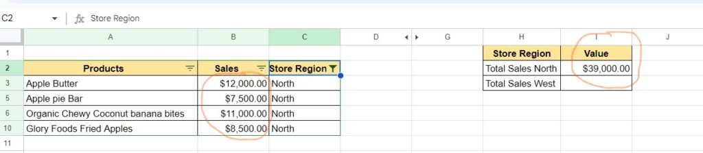
Suppose you have a sales data sheet with the following columns: Product, Sales, and Region. You want to calculate the total sales for a specific region. Here’s how you can use SUMIF to accomplish this:

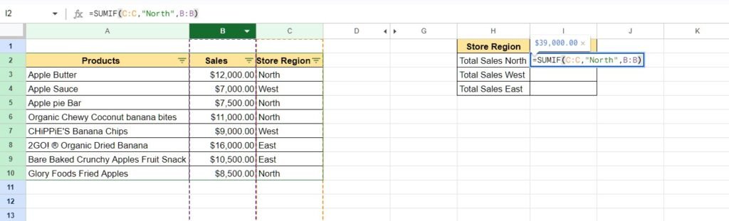
1. Select a cell where you want the total sales to appear.
2. Enter the SUMIF function: =SUMIF(C:C, “North”, B:B). This formula sums the values in column B (Sales) where the corresponding cells in column C (Region) are equal to “North”.
3. Press Enter to get the total sales for the specified region.

Example 2: google sheets SUMIF multiple criteria

In this example, let’s say you have to calculate the sum of total sales for a particular product in a particular region, so you need to put multiple criteria here. Here you have to use google sheets SUMIFS function.

SUMIF vs. SUMIFS

The SUMIF function is used to add up values based on a single criterion, while SUMIFS can compare multiple criteria.

Let’s see how you can use google sheets SUMIFS with multiple criteria:

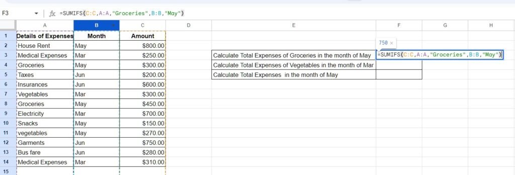
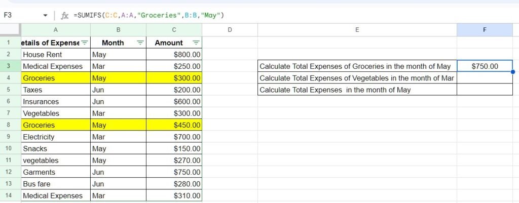
1. Select a cell where you want the total expenses to appear.
2. Enter the SUMIFS function: =SUMIF(C:C, A:A,”Groceries”, B:B, “May”). This formula sums the values in column B (Amount) where the corresponding cells in column A (Category) are equal to “Groceries” and the cells in column C (Month) is equal to “May”.
3. Press Enter to get the total expenses for the specified category and month.

Advanced Techniques with SUMIF

Apart from the basic usage of SUMIF, there are a few advanced techniques you can use to make your calculations even more powerful.

SUMIF with wildcards

You can use wildcards in your criteria to perform partial matching. The asterisk (*) represents any number of characters, while the question mark (?) represents a single character. Here’s an example:

=SUMIF(A:A, “Apples*”, B:B)

This formula sums the values in column B (Sales) where the corresponding cells in column A (Product) start with “Apples,” such as “Apple Butter” or “Apple Pie Bar.”

SUMIF with logical operators

You can also use logical operators, such as greater than (>) or less than (<), in your criteria to perform comparisons. Here’s an example:

=SUMIF(B:B, “>100”, A:A)

This formula sums the values in column A (Quantity) where the corresponding cells in column B (Price) are greater than 100.

Common Mistakes and Troubleshooting Tips

While using SUMIF, it’s quite natural you have encountered errors or unexpected results. Here are a few common mistakes and tips for troubleshooting:

• Error messages and their solutions: If you receive error messages like “#VALUE!” or “#REF!”, double-check your formula for any syntax errors or incorrect references.
• Double-checking criteria and ranges: Ensure that your criteria and ranges are correctly specified. Typos or mismatches can give you incorrect results.
• Using absolute cell references: If you want to apply the same criteria to multiple cells down the line, consider using absolute cell references by adding dollar signs ($) before the column and row references. Use Shortcut Key F4 to add $ sign.

Alternative functions to SUMIF

While SUMIF is a versatile function, there are alternatives available in Google Sheets that offer additional functionality.

Google Sheets SUMIFS

The SUMIFS function allows you to sum values based on multiple criteria simultaneously. It follows a similar syntax to SUMIF but supports multiple range and criteria pairs. This can be useful when you need to apply more complex conditions in your calculations.

Google Sheets SUMPRODUCT

The SUMPRODUCT function is another alternative to SUMIF. It allows you to multiply arrays or ranges together and then sum the results. This function can be particularly helpful when working with non-numeric criteria or when you need to perform calculations involving multiple ranges.

Conclusion

Using the SUMIF/SUMIFS function in Google Sheets can greatly simplify your data analysis and calculations. By understanding its syntax and applying various techniques, you can easily summarize data based on specific criteria. Whether you’re a business professional, student, or hobbyist, mastering SUMIF will undoubtedly enhance your productivity and decision-making capabilities.

FAQs

Can I use SUMIF to sum values in multiple sheets?

No, SUMIF is designed to work within a single sheet. If you need to sum values across multiple sheets, you can consider using other functions like SUMIFS or combining data into a single sheet.

Can I use SUMIF with dates in Google Sheets?

Yes, you can use SUMIF with dates by simply formatting your date criteria properly. For example, if your date criteria is “>=01/01/2023”, it will sum all values from the first January 2023 onwards.

Is there a limit to the number of criteria I can use in SUMIFS?

No, there is no specific limit to the number of criteria you can use in SUMIFS. You can include as many criteria as necessary to meet your requirements.

 Can I use SUMIF to sum values based on cell background color?

No, SUMIF cannot directly evaluate cell formatting. You would need to use a script or a custom formula for such requirements.

How do I use Sumif in Google Sheets with text?

Text-based criteria can be extremely useful when working with non-numeric data. SUMIF enables you to sum values based on specific text conditions, such as matching case-insensitive keywords or certain phrases. Let’s say you have a list of products, and you want to calculate the total sales of apples. Here’s how you can accomplish it:

1. Select an empty cell where you want the sum to appear.
2. Use the following formula:

=SUMIF(A2:A10, “*apples*”, B2:B10)

In this example, the asterisks work as wildcards to match any text before and after the keyword “apples”. The formula will sum all the product sales values where the product description contains the word “apples” regardless of its position within the text.