Conditional formatting in Excel is a powerful tool that allows users to visually highlight and analyze data based on specific criteria. From basic formatting to advanced techniques, mastering conditional formatting can greatly enhance your ability to interpret and present data effectively. In this beginners’ guide, I’ll delve into everything you need to know as a beginner about conditional formatting in Excel, covering its basics, advanced techniques, tips and tricks, and its significance in data analysis.
What is Conditional Formatting in Excel?
Conditional formatting is a feature in Excel that enables users to automatically format cells based on certain conditions or rules. This means that Excel applies formatting styles such as font color, background color, font style, adding icons, etc., to cells dynamically, depending on the data they contain.
Why Use Conditional Formatting in Excel?
Conditional formatting helps you draw attention to specific data points, make your spreadsheets more visually appealing, and identify patterns and outliers quickly. It saves time and makes your data analysis more efficient.
Some key benefits of using conditional formatting include:
- Enhances data visualization
- Identifies trends and patterns
- Helps in error checking and data validation
- Makes data analysis more intuitive
Where to Find Conditional Formatting in Excel?
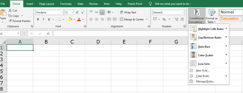
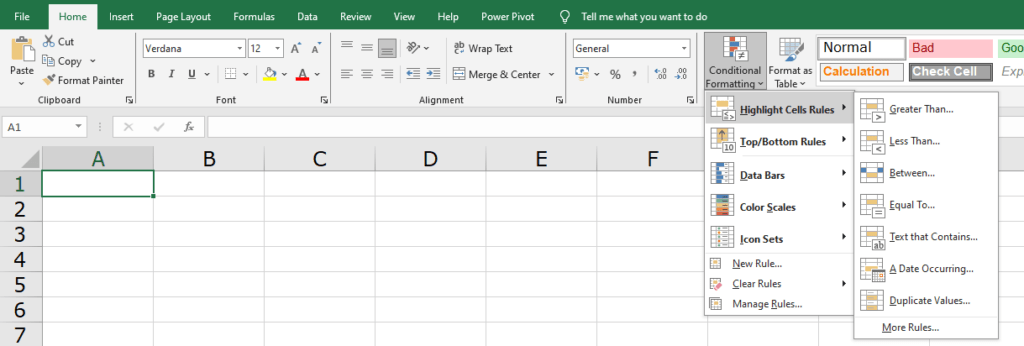
In all versions of Excel, from Excel 2010 through Excel 2019, conditional formatting resides in the same place: Home tab > Conditional formatting.

In this example, I’ll use Excel 2019, which is not the latest version like Office 365 but you’ll get all the features of conditional formatting. However, the options are essentially the same in all Excels, no matter what version is installed on your computer.
How to Apply Conditional Formatting in Excel?
Applying conditional formatting in Excel is straightforward. You can access the conditional formatting options from the Home tab on the Excel ribbon and choose from various predefined formatting rules or create custom rules based on their specific criteria.

How to Highlight Entire Row in Excel with conditional formatting?
To highlighting entire rows based on the value in a specific cell using conditional formatting in Excel by Using a Formula:
- Select the entire dataset you want to format.
- Go to the Home tab.
- In the Styles group, click on Conditional Formatting.
- Select New Rule.
- In the New Formatting Rule dialog box, choose Use a formula to determine which cells to format.
- In the formula field, enter the condition based on your desired outcome. For example:
- To highlight rows where the value in cell D1 is “Shipped”, enter: =$D1=”Shipped”
- Make sure to adjust the cell reference (D1 in this case) based on your actual data location.
- Click the Format button and choose the formatting options you want for the highlighted rows, like Fill Color.
- Click OK twice to apply the rule.
How to Copy Conditional Formatting in Excel?
There are three easy methods to copy conditional formatting in Excel. Let’s explore each one by one,
01.Using Conditional Formatting Rules Manager:
This method allows you to copy only the conditional formatting rules from one cell to another.
Follow these steps:
- Go to the Home tab.
- Click the Conditional Formatting icon.
- Select “Manage Rules…” from the expanded list of Conditional Formatting.
- In the Conditional Formatting Rules Manager dialog box:
- Expand the “Show formatting rules for” dropdown list and choose “This Worksheet”.
- Select the rule you want to copy.
- Click the “Duplicate Rule” button.
- Change the cell reference of the duplicated rule to the desired cell range.
- Click “OK” to apply the copied conditional formatting.
02. Using Format Painter:
The Format Painter is a quick way to copy formatting, including conditional formatting.
Here’s how to do :
- Click a cell that has the conditional formatting you want to copy.
- Click HOME > Format Painter.
- The pointer changes to a paintbrush.
- To copy the formatting, drag the mouse pointer across the cells or ranges where you want to apply it
03. Using Paste Special Option with Keyboard Shortcuts:
This method involves copying the entire cell format (including conditional formatting) and then pasting it.
- Select the cell with the desired formatting.
- Press Ctrl+C to copy.
- Select the target cell(s).
- Right-click and choose “Paste Special”.
- In the Paste Special dialog, select “Formats” and click “OK”.
Choose any method that suits your workflow best, and enjoy efficient conditional formatting in Excel!
How to Edit Conditional Formatting in Excel?
Often we need to change the existing conditional formatting, You can edit it by using the following steps:
- Click a cell within the range where you have an existing conditional formatting rule.
- Go to the Home tab.
- Click the Conditional Formatting button.
- Select “Manage Rules”.
- In the Conditional Formatting Rules Manager, you can:
- Edit an existing rule:
- Choose the rule you want to modify.
- Click “Edit Rule”.
- Make your changes to the rule (criteria or format).
- Click “OK” to save the edits.
- Change the order of rules (if multiple rules apply):
- Select the rule you want to resequence.
- Use the “Move Up” or “Move Down” arrow to position the rule correctly.
- Click “OK” to apply the new sequence.
How to Remove Conditional Formatting in Excel?
To remove conditional formatting in Excel, follow these steps:
- Select the cells or range of cells that have the conditional formatting you want to remove.
- Go to the “Home” tab on the Excel ribbon.
- In the “Styles” group, click on “Conditional Formatting.” This will open a dropdown menu.
- In the dropdown menu, hover over “Clear Rules.”
- You’ll see options to clear rules from the selected cells. Choose either “Clear Rules from Selected Cells” to remove conditional formatting from the selected range only, or “Clear Rules from Entire Sheet” to remove conditional formatting from the entire sheet.
- Click on the appropriate option, and the conditional formatting will be removed from the selected cells or the entire sheet, depending on your choice.
How to Use Conditional Formatting in Excel to Highlight Blank Cells?
Highlighting blank cells using conditional formatting is a useful way to draw attention to empty data points. Let’s explore couple of methods to achieve this:
Using the Built-in Rule for Blanks:
Excel provides a predefined rule for highlighting blank cells:
- Select the range where you want to highlight empty cells.
- Go to the Home tab.
- Click Conditional Formatting > New Rule.
- In the New Formatting Rule dialog box:
- Choose “Format only cells that contain”.
- Select “Blanks” from the dropdown.
- Specify the formatting (e.g., background color, font color) for blank cells.
- Click OK to apply the rule
Using the ISBLANK() Function:
This method allows more flexibility and customization:
- Select the range where you want to apply formatting.
- Go to the Home tab.
- Click Conditional Formatting > New Rule.
- Choose “Use a formula to determine which cells to format”.
- Enter the formula: =ISBLANK(D3) (replace D3 with the appropriate cell reference).
- Specify the desired formatting.
- Finally click OK to apply the rule.
